Informer (AAAI2021 Best Paper)

Contributions・サマリー

Transformerベースの長期時系列予測モデル。Transformerを使うことで長期の依存関係をとらえることができ高精度化が期待できるが、計算コストの問題があった。 そこで、Informerでは次のような改善を提案した。

• ProbSparse self-attention:

  • ナイーブなself-attentionよりも高速化

• Self-attention distilling(蒸留)：

  • self-attention層の出力のうち冗長な表現を削減することで、メモリ使用量削減

• 生成的decoder:

  • 再帰的な予測を不要とし、一度にまとめて長期系列を出力。再帰構造がなくなるため誤差の蓄積を防ぎ、計算コストも削減

実データ(ETT, Weather, ECL)での予測タスクにおいて、高精度な予測を達成した。

背景

Informer: Beyond Efficient Transformer for Long Sequence Time-Series Forecasting [1] という長期時系列予測モデルについて、著者実装をベースに解説します。この論文は、世界的に著名な機械学習系国際学会であるAAAI2021において、Best Paperに選ばれました。その後も、さまざまな深層学習ベースの時系列予測の研究においてベースライン手法として利用されています。

この論文の基本的なアイデアであるTransfomer[2] は、自然言語処理（NLP）分野で広く使われており、最近では画像処理分野においても応用が進んでいます。NLP分野では系列データを扱うために、Recurrent Neural Network(RNN)ベースのモデルが古くから提案されてきました。しかし、再帰構造をもつため並列化が難しく、長期間の依存関係を計算しようとすると、計算量が増えてしまう問題がありました。Transformerはself-attention層を組み合わせることで、この問題を解決する高速かつ高性能な手法として提案されました。

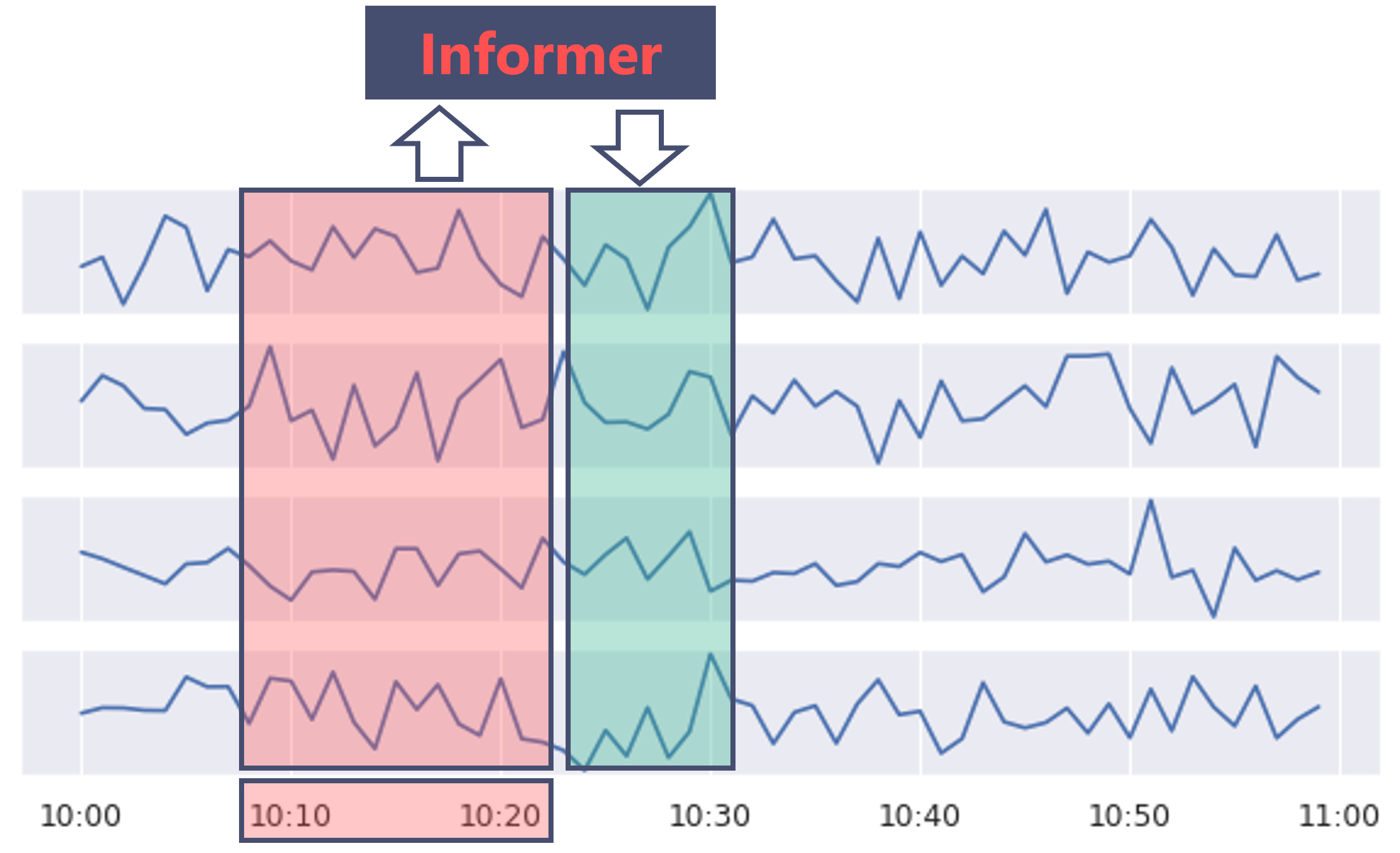
Informer はこのTransformerを時系列予測に応用したモデルです。Transformerはself-attentionのおかげで、遠い過去の特徴量にも注目できますが、それでもなお計算コストが大きいのが課題でした。具体的には、以下の課題があります。

• self-attentionの構造上、高計算コスト・高メモリ使用量（各attention層で、系列長\(L\)に対して\(O(L^2)\)）

• self-attentionを積み重ねるので、推論時のメモリ使用量の増加

• 毎回、再帰的に予測をするため、推論に時間がかかり、誤差が蓄積しやすい

そこでこの研究では、Transformerの性能を生かしつつ、計算量削減のための改善を行っています。

• ProbSparse self-attention:

  • すべてのattentionを計算するのではなく、特に重要な特徴を含んでいそうな部分のみを選択し計算（\(O(L\log L)\)）

• Self-attention distilling(蒸留)：

  • self-attention層@Encoderの出力に対して、Conv1D+Maxpooling1Dを作用させる。冗長な表現を削減することで、メモリ使用量削減

• 生成的decoder:

  • 再帰的な予測を不要とし、一度にまとめて長期系列を出力。再帰構造がなくなるため誤差の蓄積を防ぎ、計算コストも削減

本記事では、それぞれの構成要素を解説し、ETTデータセット を用いた検証を行います。

注意

• 本記事はコード量が多いため、主要な部分以外は折り畳み表示しています。また、GPUを使わないと学習にかなりの時間がかかる場合があります。

• 著者実装 （Apache License 2.0）をベースとして、解説に必要な部分だけを抽出し、多少の修正とドキュメントを充実させたものです。

• Transofomerの解説は、素晴らしい解説がすでに多く執筆されているため省略します。

ライブラリ読み込み

Show code cell content

Hide code cell content

import sys
import platform
from pathlib import Path
import random
from typing import Union, List
import numpy as np
import pandas as pd
from sklearn.preprocessing import StandardScaler
import matplotlib.pyplot as plt

# import japanize_matplotlib
import seaborn

import torch
from torch.utils.data import Dataset, DataLoader
from torch import optim
from torch import nn
import torch.nn.functional as F
from pandas.tseries import offsets
from pandas.tseries.frequencies import to_offset

from omegaconf import OmegaConf

seaborn.set_theme(font="Noto Sans CJK JP")  # グラフの日本語フォント化

# 乱数の固定
seed = 123

random.seed(seed)
np.random.seed(seed)
torch.manual_seed(seed)
torch.backends.cudnn.benchmark = False
torch.backends.cudnn.deterministic = True

# 主要ライブラリのバージョン
print(f"Python version: {platform.python_version()}")
print(f"PyTorch version: {torch.__version__}")
print(f"Pandas version: {pd.__version__}")
print(f"Numpy version: {np.__version__}")

Python version: 3.11.8
PyTorch version: 2.8.0+cu128
Pandas version: 2.3.2
Numpy version: 2.2.0

モデル

モデルの概略図を示します。

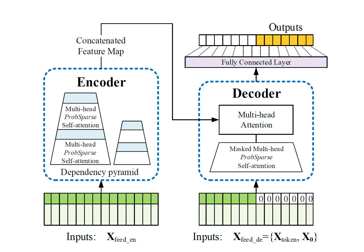
論文Figure2より引用。 緑色の系列が入力データで、濃いほうが時系列の値（=token）、薄いほうが対応する時刻情報。Encoderでは入力　\(\mathbf{X}_\mathrm{feed\_en}\)　から、ProbSparse Self-attentionを通して系列間の依存関係を考慮した特徴表現を得る。Decoderには、指定された時刻より先の値を予測することを指示する start token \(\mathbf{X}_\mathrm{token}\) と、 予測対象と同じ長さのゼロ埋めtoken \(\mathbf{X}_\mathrm{0}\)（ただし時刻情報だけは保持） とを結合した　\(\mathbf{X}_\mathrm{feed\_de}\) を入力する。EncoderとDecoderの具体的な入力については、Decoder節の図を参照。Encoder, Decoderそれぞれで得られた特徴表現から予測を行う（オレンジの系列）。

基本的な構造はTransformerを継承しています。つまり、入力データは（図中には描かれていませんが）Embedding層で埋め込み表現に変換されたのち、self-attentionをベースとしたencoder-decoder構造に入力されます。encoderでは時系列の特徴量を計算し、decoderでは、この特徴量をもちいて未来の部分を予測します。

ここでは、Informerを構成する各コンポーネント、Embedding, ProbSparse self-attention, Encoder, Decoder について解説します。なお、InformerではTransfomerと語彙をそろえるため、時系列の値自体（これ単体では時刻情報を含まない）を token と呼ぶこととします。

Embedding

データをモデルに入力するために変換を行います。通常のTransfomerモデルでは、系列データの順序関係（例えば単語の並び順）を位置エンコーディング（positional encoding） で表現します。Informerで興味の対象とする時系列データでは、単なる順序関係だけではなく、日付時刻も重要な情報です。

そこで、データの値、順序関係、時刻情報それぞれをPositional embedding, Token embedding, Time feature embeddingで変換し、入力表現とします。

Positional Embedding

Trasformerの場合と同様に、\(\sin, \cos\) 関数を用いて位置エンコーディングを施します。

\[\begin{align*} \mathrm{PE}_{(pos, 2j)} &= \sin (pos/(2L_x)^{2j/d_{model}}) \\ \mathrm{PE}_{(pos, 2j+1)} &= \cos (pos/(2L_x)^{2j/d_{model}}) \end{align*}\]

• \(pos\): 入力系列のトークン位置。時系列の文脈では時刻方向のindex番号に対応

• \(j\in \{1,\cdots, \lfloor d_{model}/2 \rfloor \}\): 次元方向のインデックス番号.

• \(L_x\): 入力系列の長さ

• \(d_{model}\): 変換後の次元数

※ 著者実装では、クラス名がPositionalEmbedding として定義されていますが学習可能なパラメータで変換しているわけではないので、実態としてはencodingだと考えられます。

class PositionalEmbedding(nn.Module):
    def __init__(self, d_model: int, max_len: int = 5000):
        super(PositionalEmbedding, self).__init__()
        # Compute the positional encodings once in log space.
        pe = torch.zeros(max_len, d_model).float()
        pe.require_grad = False

        position = torch.arange(0, max_len).float().unsqueeze(1)
        div_term = (
            torch.arange(0, d_model, 2).float() * -(np.log(10000.0) / d_model)
        ).exp()

        pe[:, 0::2] = torch.sin(position * div_term)
        pe[:, 1::2] = torch.cos(position * div_term)

        pe = pe.unsqueeze(0)
        self.register_buffer("pe", pe)

    def forward(self, x):
        return self.pe[:, : x.size(1)]

Token Embedding

こちらもTransformerと同様、各時刻における値(=token)を一次元畳み込み層で埋め込みます。

class TokenEmbedding(nn.Module):
    def __init__(self, c_in: int, d_model: int):
        super(TokenEmbedding, self).__init__()
        padding = 1 if torch.__version__ >= "1.5.0" else 2
        self.tokenConv = nn.Conv1d(
            in_channels=c_in,
            out_channels=d_model,
            kernel_size=3,
            padding=padding,
            padding_mode="circular",
        )
        for m in self.modules():
            if isinstance(m, nn.Conv1d):
                nn.init.kaiming_normal_(
                    m.weight, mode="fan_in", nonlinearity="leaky_relu"
                )

    def forward(self, x):
        x = self.tokenConv(x.permute(0, 2, 1)).transpose(1, 2)
        return x

Time Feature Embedding

日付時刻情報を線形変換（学習可能）で埋め込みます。ここで入力される時刻情報は、関数time_features()で\([-0.5, 0.5]\)に変換された値です。 また、入力次元はデータのサンプリング間隔に依存します。

Show code cell content

Hide code cell content

class TimeFeature:
    def __init__(self):
        pass

    def __call__(self, index: pd.DatetimeIndex) -> np.ndarray:
        pass

    def __repr__(self):
        return self.__class__.__name__ + "()"


class SecondOfMinute(TimeFeature):
    """Minute of hour encoded as value between [-0.5, 0.5]"""

    def __call__(self, index: pd.DatetimeIndex) -> np.ndarray:
        return index.second / 59.0 - 0.5


class MinuteOfHour(TimeFeature):
    """Minute of hour encoded as value between [-0.5, 0.5]"""

    def __call__(self, index: pd.DatetimeIndex) -> np.ndarray:
        return index.minute / 59.0 - 0.5


class HourOfDay(TimeFeature):
    """Hour of day encoded as value between [-0.5, 0.5]"""

    def __call__(self, index: pd.DatetimeIndex) -> np.ndarray:
        return index.hour / 23.0 - 0.5


class DayOfWeek(TimeFeature):
    """Hour of day encoded as value between [-0.5, 0.5]"""

    def __call__(self, index: pd.DatetimeIndex) -> np.ndarray:
        return index.dayofweek / 6.0 - 0.5


class DayOfMonth(TimeFeature):
    """Day of month encoded as value between [-0.5, 0.5]"""

    def __call__(self, index: pd.DatetimeIndex) -> np.ndarray:
        return (index.day - 1) / 30.0 - 0.5


class DayOfYear(TimeFeature):
    """Day of year encoded as value between [-0.5, 0.5]"""

    def __call__(self, index: pd.DatetimeIndex) -> np.ndarray:
        return (index.dayofyear - 1) / 365.0 - 0.5


class MonthOfYear(TimeFeature):
    """Month of year encoded as value between [-0.5, 0.5]"""

    def __call__(self, index: pd.DatetimeIndex) -> np.ndarray:
        return (index.month - 1) / 11.0 - 0.5


class WeekOfYear(TimeFeature):
    """Week of year encoded as value between [-0.5, 0.5]"""

    def __call__(self, index: pd.DatetimeIndex) -> np.ndarray:
        return (index.isocalendar().week - 1) / 52.0 - 0.5


def time_features_from_frequency_str(freq_str: str) -> List[TimeFeature]:
    """
    Returns a list of time features that will be appropriate for the given frequency string.
    Parameters
    ----------
    freq_str
        Frequency string of the form [multiple][granularity] such as "12H", "5min", "1D" etc.
    """

    features_by_offsets = {
        offsets.YearEnd: [],
        offsets.QuarterEnd: [MonthOfYear],
        offsets.MonthEnd: [MonthOfYear],
        offsets.Week: [DayOfMonth, WeekOfYear],
        offsets.Day: [DayOfWeek, DayOfMonth, DayOfYear],
        offsets.BusinessDay: [DayOfWeek, DayOfMonth, DayOfYear],
        offsets.Hour: [HourOfDay, DayOfWeek, DayOfMonth, DayOfYear],
        offsets.Minute: [
            MinuteOfHour,
            HourOfDay,
            DayOfWeek,
            DayOfMonth,
            DayOfYear,
        ],
        offsets.Second: [
            SecondOfMinute,
            MinuteOfHour,
            HourOfDay,
            DayOfWeek,
            DayOfMonth,
            DayOfYear,
        ],
    }

    offset = to_offset(freq_str)

    for offset_type, feature_classes in features_by_offsets.items():
        if isinstance(offset, offset_type):
            return [cls() for cls in feature_classes]

    supported_freq_msg = f"""
    Unsupported frequency {freq_str}
    The following frequencies are supported:
        Y   - yearly
            alias: A
        M   - monthly
        W   - weekly
        D   - daily
        B   - business days
        H   - hourly
        T   - minutely
            alias: min
        S   - secondly
    """
    raise RuntimeError(supported_freq_msg)

def time_features(dates: np.array, freq: str = "h") -> np.array:
    """時間特徴量を、指定されたサンプリング間隔に応じて変換。それぞれの値は[-0.5, 0.5]に正規化されている。

    > * Q - [month]
    > * M - [month]
    > * W - [Day of month, week of year]
    > * D - [Day of week, day of month, day of year]
    > * B - [Day of week, day of month, day of year]
    > * H - [Hour of day, day of week, day of month, day of year]
    > * T - [Minute of hour*, hour of day, day of week, day of month, day of year]
    > * S - [Second of minute, minute of hour, hour of day, day of week, day of month, day of year]
    *minute returns a number from 0-3 corresponding to the 15 minute period it falls into.

    ※ 著者実装では、学習可能なパラメータを持たせない（単なるルックアップテーブルとして保持）場合の実装もあるが、ここでは省略。

    Parameters
    ----------
    dates : np.array
        日時が格納されている配列
    freq : str, optional
        サンプリング間隔, by default 'h'
        指定方法はpandasのdatetimeの記法に従う。
        例: "1h", "2h", "3D", etc...

    Returns
    -------
    np.array
        変換後の時間特徴量
        【例】: 2023-5-16 19:00 -> [Hour of day, day of week, day of month, day of year] の4次元
    """
    dates = pd.to_datetime(dates.date.values)
    ret = np.vstack(
        [feat(dates) for feat in time_features_from_frequency_str(freq)]
    ).transpose(1, 0)
    return ret


# 日付変換の例
df_stamp = pd.DataFrame(
    {"date": [pd.to_datetime("2023-5-16 19:00"), pd.to_datetime("2023-5-16 20:00")]}
)
data_stamp = time_features(df_stamp, freq="h")
print(data_stamp)

[[ 0.32608696 -0.33333333  0.         -0.13013699]
 [ 0.36956522 -0.33333333  0.         -0.13013699]]

class TimeFeatureEmbedding(nn.Module):
    def __init__(self, d_model: int, freq: str = "h"):
        super(TimeFeatureEmbedding, self).__init__()

        freq_map = {"h": 4, "t": 5, "s": 6, "m": 1, "a": 1, "w": 2, "d": 3, "b": 3}
        d_inp = freq_map[freq]
        self.embed = nn.Linear(d_inp, d_model)

    def forward(self, x):
        return self.embed(x)

入力表現まとめ

Positional Embedding, Token Embedding, TimeFeature Embedding をまとめ、足し合わせることで、Data Embeddingで埋め込み表現を得ます。

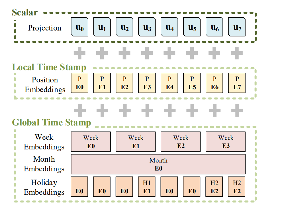
論文中Figure 6より。Scalar, Local Time Stamp, Global Time StampがそれぞれTokenEmbedding, PositionalEmbedding, TimeFeatureEmbeddingに対応。

class DataEmbedding(nn.Module):
    def __init__(self, c_in, d_model, freq="h", dropout=0.1):
        super(DataEmbedding, self).__init__()

        self.value_embedding = TokenEmbedding(c_in=c_in, d_model=d_model)
        self.position_embedding = PositionalEmbedding(d_model=d_model)
        self.temporal_embedding = TimeFeatureEmbedding(d_model=d_model, freq=freq)

        self.dropout = nn.Dropout(p=dropout)

    def forward(self, x, x_mark):
        x = (
            self.value_embedding(x)
            + self.position_embedding(x)
            + self.temporal_embedding(x_mark)
        )

        return self.dropout(x)

ProbSparse self-attention

通常のself-attention機構では、Query;\(\mathbf{Q} \in \mathbb{R}^{L_Q\times d}\), Key; \(\mathbf{K} \in \mathbb{R}^{L_K\times d}\), Value; \(\mathbf{V} \in \mathbb{R}^{L_V\times d}\) をもちいて入力表現間の関連度attention; \(A\) を計算し、これを新しい表現として次の層に入力します。\(L_Q, L_K, L_V, d\) はそれぞれ、Query長, Key長, Value長, 入力次元（列方向）です。

\[ A(\mathbf{Q}, \mathbf{K}, \mathbf{V}) = \mathrm{Softmax} ( \frac{\mathbf{QK}^T}{\sqrt{d}} ) \mathbf{V} \]

Attention行列\(\mathbf{A}\)の\(i\)行目の計算は

\[\begin{align*} A(\mathbf{q}_i, \mathbf{K}, \mathbf{V}) &= \sum_j \frac{\exp(\mathbf{q}_i \mathbf{k}_j / \sqrt d)}{\sum_l \exp(\mathbf{q}_i\mathbf{k}_l / \sqrt d)} \mathbf{v}_j \\ &= \mathbb E _{p(\mathbf{k}_j|\mathbf{q}_i)} [\mathbf{v}_j] \end{align*}\]

\[ p(\mathbf{k}_j|\mathbf{q}_i) = \frac{\exp(\mathbf{q}_i \mathbf{k}_j / \sqrt d)}{\sum_l \exp(\mathbf{q}_i\mathbf{k}_l / \sqrt d)} \]

と書くことができます。\(p\)は規格化されているので、各value \(\mathbf{v}_j\) に対する重みづけとみることができます。

ここで、行列積\(\mathbf{QK}^T\)の計算に\(\mathcal{O}(L_Q L_K)\)がかかることがself-attention、ひいてはこれを多層に積み上げるTransfomerの欠点です（実装上は\(L_Q=L_K=L_V=L\)とすることが多いので\(\mathcal{O}(L^2)\)）。

Query Sparsity Measurement

計算コストを下げるために、self-attentionのうち重要でないものは無視することが基本的な考え方です（下図参照）。

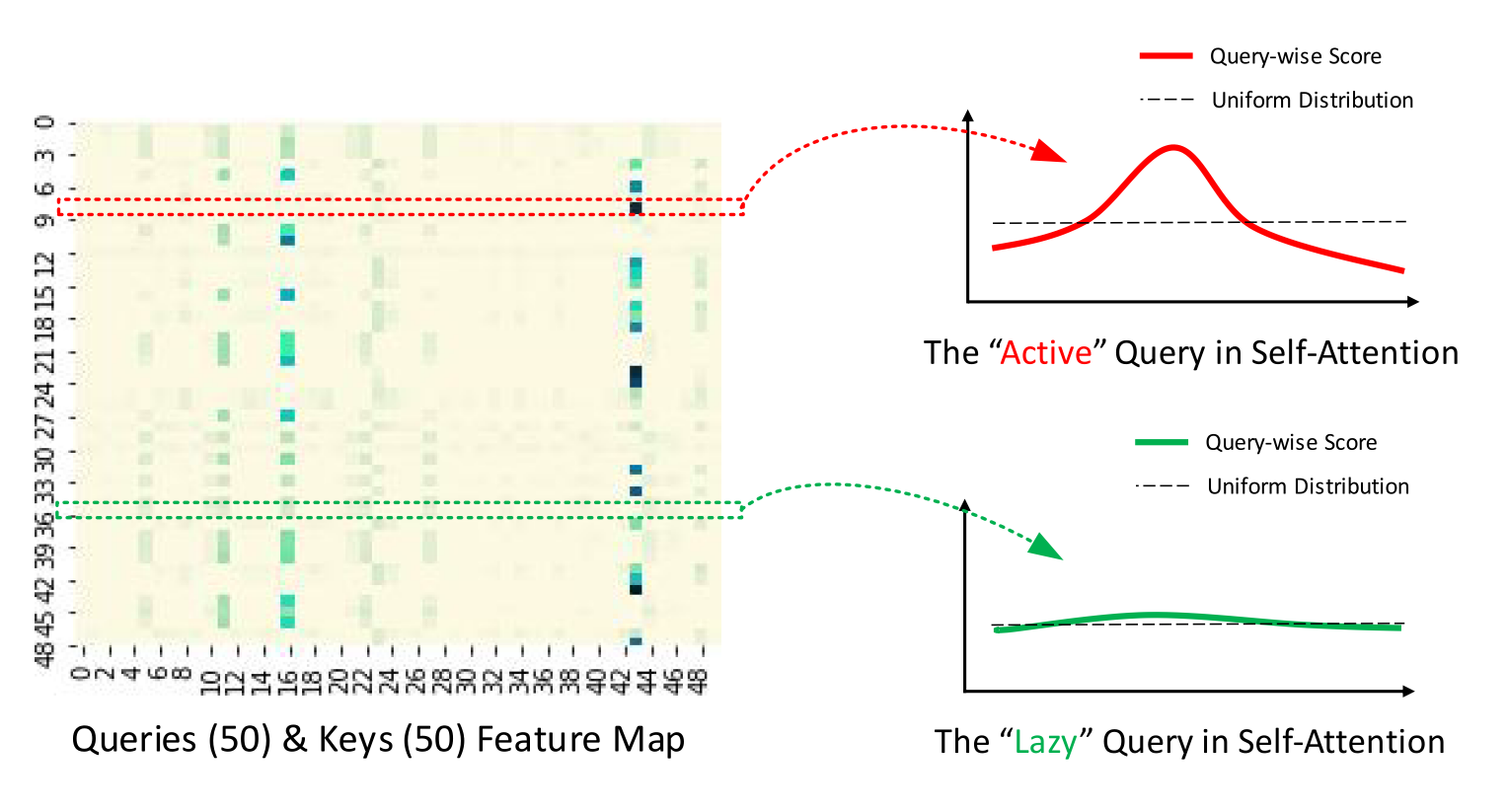
ProbSparse attentionのイメージ図（著者実装GitHubより）。Attention Map \(\mathbf{QK}^T\)を可視化した例で、色が濃いほどquery-key値が大きいことを示す。Query方向に切断してみる（赤と緑の例示）と、より重要なqueryでは、一部でこの値が大きくなっており一様分布からは遠くなることがイメージできる。

もし、\(p(\mathbf{k}_j|\mathbf{q}_i)\)が一様分布\(q(k_j|q_i)=1/L_K\) に近ければ、対して影響がなく、入力から無視できると考えられます。そこで、重要度を\(p, q\)のKL divergence

\[ KL(q||p) = \ln \sum_{j=1}^{L_K} e^{\mathbf{q}_i \mathbf{k}_j^T / \sqrt{d}} - \frac{1}{L_K} \sum_{j=1}^{L_K} \frac{\mathbf{q}_i \mathbf{k}_j^T}{\sqrt{d}} - \ln L_K \]

をもとに、定数項\(\ln L_K\)を無視して、query sparsity measurement \(M\)として定義します。

(1)\[ M(\mathbf{q}_i, \mathbf{K}) = \ln \sum_{j=1}^{L_K} e^{\mathbf{q}_i \mathbf{k}_j^T / \sqrt{d}} - \frac{1}{L_K} \sum_{j=1}^{L_K} \frac{\mathbf{q}_i \mathbf{k}_j^T}{\sqrt{d}} \]

この\(M\)が大きいほど、より重要な情報をもった行列積のペアである可能性が高いことを意味します。

したがって、この指標に基づいて重要な\(u\)個(Top-\(u\))のqueryだけを使ってattentionを計算することとします。

\[ A(\mathbf{Q}, \mathbf{K}, \mathbf{V}) = \mathrm{Softmax} ( \frac{\mathbf{\bar{Q} K}^T}{\sqrt{d}} ) \mathbf{V} \]

\(\bar{\mathbf Q}\) はTop-\(u\)個のqueryだけを含む疎行列です。\(u\)の決め方は、sampling factor \(c\)として、\(u=c\cdot\ln L_Q\) と決め打ちでおくこととします（\(c\)はハイパーパラメーターで大きい値を設定すればより多くのqueryをとってくる）。このとき、それぞれのquery-keyについて、\(\mathcal O (\ln L_Q)\) の行列積を計算すればよく、その時のメモリ使用量も\(\mathcal O (L_K \ln L_Q)\)になります。

しかし、結局のところTop-\(u\)の順位付けをするために、\(M\)をすべての組について行列演算したのでは \(\mathcal O (L_Q L_K)\) からは逃れられません。加えて(1)の右辺第1項のLog-Sum-Exp（LSE）は数値計算上も安定性の課題を抱えています。

証明は論文Appendix D.1に譲るとして、\(M\)は次のように緩和することができます。

\[ \bar M(\mathbf{q}_i, \mathbf{K}) = \max_j \frac{\mathbf{q}_i \mathbf{k}_j^T}{\sqrt{d}} - \frac{1}{L_K} \sum_{j=1}^{L_K} \frac{\mathbf{q}_i \mathbf{k}_j^T}{\sqrt{d}} \]

\(\bar M(\mathbf{q}_i, \mathbf{K})\) はAttention Scoreの最大値から、平均値を引くことで、その重要度を測る形になっています。直感的にも、一様分布との差異は、わざわざKL divergenceを計算しなくとも、最大値と平均との差でも表せそうです（一様分布に近ければ最大値と平均値の差がなくなるため）。また\(\max\) の計算もLSEより数値的に安定していることもメリットです。

さらに、Appendix D.2より、\(\mathbf{q}_i\) にたいしてkeyをすべて計算する必要はなく、keyを\(\ln L_K\) 個サンプリングしてくれば、\(\bar M(\mathbf{q}_i, \mathbf{K}) \) を見積もることができます^※。この場合の計算量は\(\mathbf{q}_i\) が\(L_Q\)行あるので、\(\mathcal O (L_Q \ln L_K)\) です。

以上より、\(\bar M\) を計算し、そのうちTop-\(u\) 個のqueryだけを使ってAttention Mapを計算します。前述の通り、実用上は \(L_Q=L_K=L\) として、提案手法ProbSparse self-attentionの計算量は\(\mathcal O (L \ln L)\) になります。

注釈

※ 論文中では、必要なサンプル数を\(U=L_K \ln L_Q\) として書かれていますが、著者実装は \(U=c \cdot L_Q \ln L_K\)　で、また、解釈的にも間引くのはkey方向のため\(\ln L_K\) が正しいと思われます。

class ProbMask:
    def __init__(self, B, H, L, index, scores, device="cpu"):
        _mask = torch.ones(L, scores.shape[-1], dtype=torch.bool).to(device).triu(1)
        _mask_ex = _mask[None, None, :].expand(B, H, L, scores.shape[-1])
        indicator = _mask_ex[
            torch.arange(B)[:, None, None], torch.arange(H)[None, :, None], index, :
        ].to(device)
        self._mask = indicator.view(scores.shape).to(device)

    @property
    def mask(self):
        return self._mask


class ProbAttention(nn.Module):
    def __init__(
        self,
        mask_flag=True,
        factor=5,
        scale=None,
        attention_dropout=0.1,
        output_attention=False,
    ):
        super(ProbAttention, self).__init__()
        self.factor = factor
        self.scale = scale
        self.mask_flag = mask_flag
        self.output_attention = output_attention
        self.dropout = nn.Dropout(attention_dropout)

    def _prob_QK(self, Q, K, sample_k, n_top):  # n_top: c*ln(L_q)
        # Q [B, H, L, D]
        B, H, L_K, E = K.shape
        _, _, L_Q, _ = Q.shape

        # calculate the sampled Q_K
        K_expand = K.unsqueeze(-3).expand(B, H, L_Q, L_K, E)
        index_sample = torch.randint(
            L_K, (L_Q, sample_k)
        )  # real U = U_part(factor*ln(L_k))*L_q
        K_sample = K_expand[:, :, torch.arange(L_Q).unsqueeze(1), index_sample, :]
        Q_K_sample = torch.matmul(Q.unsqueeze(-2), K_sample.transpose(-2, -1)).squeeze(
            -2
        )

        # find the Top_k query with sparisty measurement
        M = Q_K_sample.max(-1)[0] - torch.div(Q_K_sample.sum(-1), L_K)
        M_top = M.topk(n_top, sorted=False)[1]

        # use the reduced Q to calculate Q_K
        Q_reduce = Q[
            torch.arange(B)[:, None, None], torch.arange(H)[None, :, None], M_top, :
        ]  # factor*ln(L_q)
        Q_K = torch.matmul(Q_reduce, K.transpose(-2, -1))  # factor*ln(L_q)*L_k

        return Q_K, M_top

    def _get_initial_context(self, V, L_Q):
        B, H, L_V, D = V.shape
        if not self.mask_flag:
            # V_sum = V.sum(dim=-2)
            V_sum = V.mean(dim=-2)
            contex = V_sum.unsqueeze(-2).expand(B, H, L_Q, V_sum.shape[-1]).clone()
        else:  # use mask
            assert L_Q == L_V  # requires that L_Q == L_V, i.e. for self-attention only
            contex = V.cumsum(dim=-2)
        return contex

    def _update_context(self, context_in, V, scores, index, L_Q, attn_mask):
        B, H, L_V, D = V.shape

        if self.mask_flag:
            attn_mask = ProbMask(B, H, L_Q, index, scores, device=V.device)
            scores.masked_fill_(attn_mask.mask, -np.inf)

        attn = torch.softmax(scores, dim=-1)  # nn.Softmax(dim=-1)(scores)

        context_in[
            torch.arange(B)[:, None, None], torch.arange(H)[None, :, None], index, :
        ] = torch.matmul(attn, V).type_as(context_in)
        if self.output_attention:
            attns = (torch.ones([B, H, L_V, L_V]) / L_V).type_as(attn).to(attn.device)
            attns[
                torch.arange(B)[:, None, None], torch.arange(H)[None, :, None], index, :
            ] = attn
            return (context_in, attns)
        else:
            return (context_in, None)

    def forward(self, queries, keys, values, attn_mask):
        B, L_Q, H, D = queries.shape
        _, L_K, _, _ = keys.shape

        queries = queries.transpose(2, 1)
        keys = keys.transpose(2, 1)
        values = values.transpose(2, 1)

        U_part = self.factor * np.ceil(np.log(L_K)).astype("int").item()  # c*ln(L_k)
        u = self.factor * np.ceil(np.log(L_Q)).astype("int").item()  # c*ln(L_q)

        U_part = U_part if U_part < L_K else L_K
        u = u if u < L_Q else L_Q

        scores_top, index = self._prob_QK(queries, keys, sample_k=U_part, n_top=u)

        # add scale factor
        scale = self.scale or 1.0 / np.sqrt(D)
        if scale is not None:
            scores_top = scores_top * scale
        # get the context
        context = self._get_initial_context(values, L_Q)
        # update the context with selected top_k queries
        context, attn = self._update_context(
            context, values, scores_top, index, L_Q, attn_mask
        )

        return context.transpose(2, 1).contiguous(), attn

ここで、encoder-decoderモデルの構築に必要な、通常のattention層も用意しておきます。

Show code cell content

Hide code cell content

class TriangularCausalMask:
    def __init__(self, B, L, device="cpu"):
        mask_shape = [B, 1, L, L]
        with torch.no_grad():
            self._mask = torch.triu(
                torch.ones(mask_shape, dtype=torch.bool), diagonal=1
            ).to(device)

    @property
    def mask(self):
        return self._mask


class FullAttention(nn.Module):
    def __init__(
        self,
        mask_flag=True,
        factor=5,
        scale=None,
        attention_dropout=0.1,
        output_attention=False,
    ):
        super(FullAttention, self).__init__()
        self.scale = scale
        self.mask_flag = mask_flag
        self.output_attention = output_attention
        self.dropout = nn.Dropout(attention_dropout)

    def forward(self, queries, keys, values, attn_mask):
        B, L, H, E = queries.shape
        _, S, _, D = values.shape
        scale = self.scale or 1.0 / np.sqrt(E)

        scores = torch.einsum("blhe,bshe->bhls", queries, keys)
        if self.mask_flag:
            if attn_mask is None:
                attn_mask = TriangularCausalMask(B, L, device=queries.device)

            scores.masked_fill_(attn_mask.mask, -np.inf)

        A = self.dropout(torch.softmax(scale * scores, dim=-1))
        V = torch.einsum("bhls,bshd->blhd", A, values)

        if self.output_attention:
            return (V.contiguous(), A)
        else:
            return (V.contiguous(), None)


class AttentionLayer(nn.Module):
    def __init__(
        self, attention, d_model, n_heads, d_keys=None, d_values=None, mix=False
    ):
        super(AttentionLayer, self).__init__()

        d_keys = d_keys or (d_model // n_heads)
        d_values = d_values or (d_model // n_heads)

        self.inner_attention = attention
        self.query_projection = nn.Linear(d_model, d_keys * n_heads)
        self.key_projection = nn.Linear(d_model, d_keys * n_heads)
        self.value_projection = nn.Linear(d_model, d_values * n_heads)
        self.out_projection = nn.Linear(d_values * n_heads, d_model)
        self.n_heads = n_heads
        self.mix = mix

    def forward(self, queries, keys, values, attn_mask):
        B, L, _ = queries.shape
        _, S, _ = keys.shape
        H = self.n_heads

        queries = self.query_projection(queries).view(B, L, H, -1)
        keys = self.key_projection(keys).view(B, S, H, -1)
        values = self.value_projection(values).view(B, S, H, -1)

        out, attn = self.inner_attention(queries, keys, values, attn_mask)
        if self.mix:
            out = out.transpose(2, 1).contiguous()
        out = out.view(B, L, -1)

        return self.out_projection(out), attn

Encoder

入力される時系列データから、ProbSparse self-attention層を通すことで長期間の依存関係を獲得します。

Self-attention Distilling

ProbSparse self-attentionで得られた特徴量マップの中には冗長なvalueが含まれていることが考えられます。そのため、各層の間でdistilling(蒸留)を行い、より優れた特徴量を抽出、計算量を削減します。ここでは、先行研究でも用いられているように、self-attention層を出るたびに1次元畳み込み（kernel size=3）とMaxPooling(stride=2)の操作を行います。第\(j\)-attention層での出力を \([\mathbf{X}_j]_\mathrm{AB}\) として、次の\(j+1\)層への入力 \(\mathbf{X}_{j+1}\) は次のような操作が行われます（活性化関数としてELUを使用）。

\[ \mathbf{X}_{j+1} = \mathrm{MaxPool} \left(\mathrm{ELU} \left(\mathrm{Conv1d}\left( [\mathbf{X}_j]_\mathrm{AB} \right) \right) \right) \]

これにより、各層を出るたびに半分のサイズにダウンサンプリングされ、合計のメモリ使用量は\(\mathcal O ((2-\epsilon) L \log L)\) になります。

class ConvLayer(nn.Module):
    def __init__(self, c_in):
        super(ConvLayer, self).__init__()
        padding = 1 if torch.__version__ >= "1.5.0" else 2
        self.downConv = nn.Conv1d(
            in_channels=c_in,
            out_channels=c_in,
            kernel_size=3,
            padding=padding,
            padding_mode="circular",
        )
        self.norm = nn.BatchNorm1d(c_in)
        self.activation = nn.ELU()
        self.maxPool = nn.MaxPool1d(kernel_size=3, stride=2, padding=1)

    def forward(self, x):
        x = self.downConv(x.permute(0, 2, 1))
        x = self.norm(x)
        x = self.activation(x)
        x = self.maxPool(x)
        x = x.transpose(1, 2)
        return x


class EncoderLayer(nn.Module):
    def __init__(self, attention, d_model, d_ff=None, dropout=0.1, activation="relu"):
        super(EncoderLayer, self).__init__()
        d_ff = d_ff or 4 * d_model
        self.attention = attention
        self.conv1 = nn.Conv1d(in_channels=d_model, out_channels=d_ff, kernel_size=1)
        self.conv2 = nn.Conv1d(in_channels=d_ff, out_channels=d_model, kernel_size=1)
        self.norm1 = nn.LayerNorm(d_model)
        self.norm2 = nn.LayerNorm(d_model)
        self.dropout = nn.Dropout(dropout)
        self.activation = F.relu if activation == "relu" else F.gelu

    def forward(self, x, attn_mask=None):
        # x [B, L, D]
        # x = x + self.dropout(self.attention(
        #     x, x, x,
        #     attn_mask = attn_mask
        # ))
        new_x, attn = self.attention(x, x, x, attn_mask=attn_mask)
        x = x + self.dropout(new_x)

        y = x = self.norm1(x)
        y = self.dropout(self.activation(self.conv1(y.transpose(-1, 1))))
        y = self.dropout(self.conv2(y).transpose(-1, 1))

        return self.norm2(x + y), attn


class Encoder(nn.Module):
    def __init__(self, attn_layers, conv_layers=None, norm_layer=None):
        super(Encoder, self).__init__()
        self.attn_layers = nn.ModuleList(attn_layers)
        self.conv_layers = (
            nn.ModuleList(conv_layers) if conv_layers is not None else None
        )
        self.norm = norm_layer

    def forward(self, x, attn_mask=None):
        # x [B, L, D]
        attns = []
        if self.conv_layers is not None:
            for attn_layer, conv_layer in zip(self.attn_layers, self.conv_layers):
                x, attn = attn_layer(x, attn_mask=attn_mask)
                x = conv_layer(x)
                attns.append(attn)
            x, attn = self.attn_layers[-1](x, attn_mask=attn_mask)
            attns.append(attn)
        else:
            for attn_layer in self.attn_layers:
                x, attn = attn_layer(x, attn_mask=attn_mask)
                attns.append(attn)

        if self.norm is not None:
            x = self.norm(x)

        return x, attns

Decoder

DecoderはTransfomerで提案されたものと同等の構造です。時刻\(t\)のDecode入力は

\[ \mathbf{X}_\mathrm{de}^t = \mathrm{Concat} (\mathbf{X}_\mathrm{token}^t, \mathbf{X}_\mathrm{0}^t) \in \mathbb{R}^{L_{\mathrm(token)+L_y}\times d_\mathrm{model}} \]

です。\(\mathbf{X}_\mathrm{token}^t\) はstart tokenで、この時刻より先の値を予測することを指示します。\(\mathbf{X}_\mathrm{0}^t\) は予測対象と同じ長さのベクトルで、時刻情報のみが含まれています。入力データにそのまま予測対象が入ってしまうとカンニングすることになってしまうので、データ部分は0で置き換えられています。それぞれの入出力系列の対応関係は下図のようになっています。

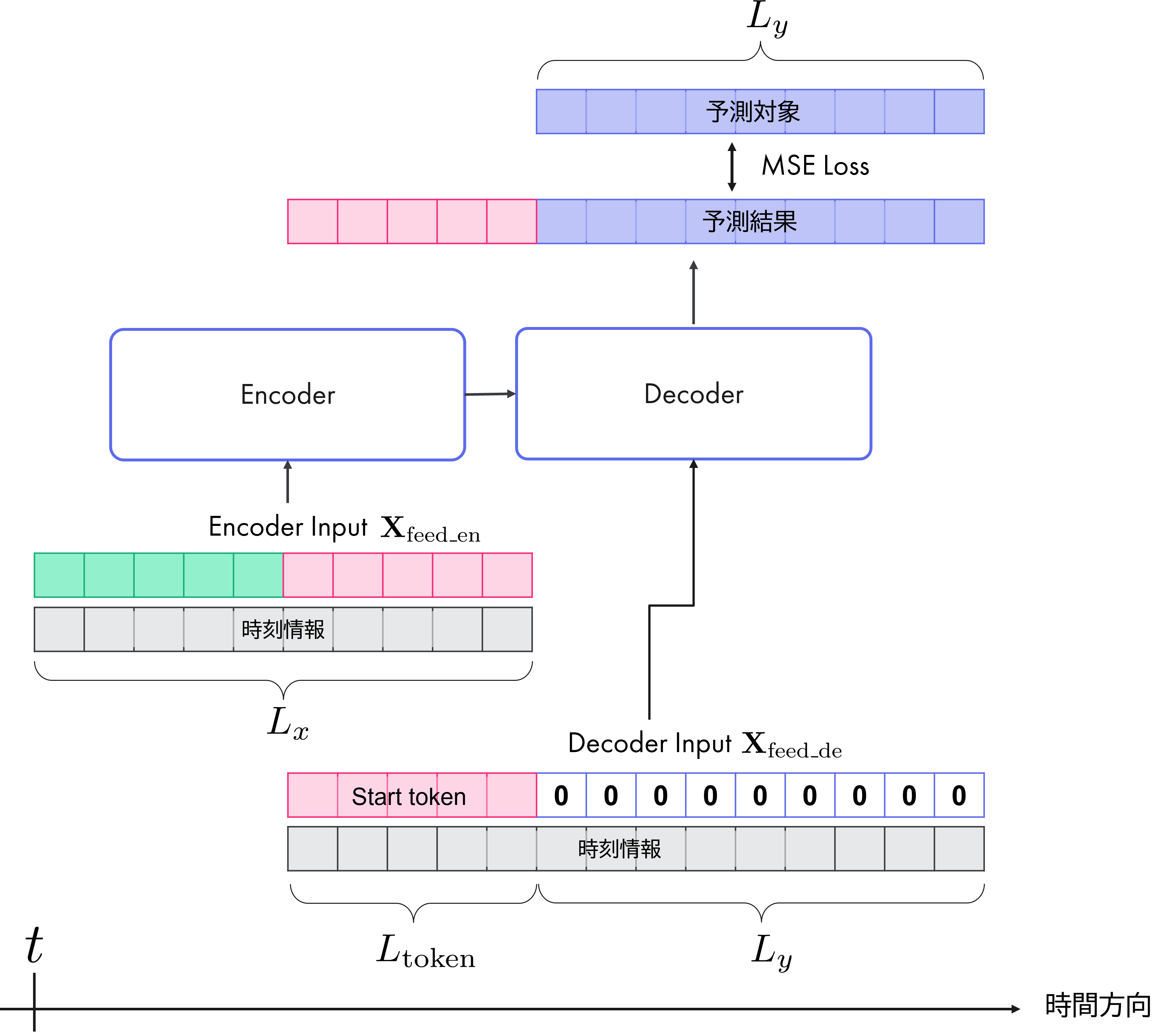
モデルへの入力のイメージ。ある時刻 \(t\) を始点として、encoder入力系列 \(\mathbf{X}_\mathrm{en}^t\) は \(L_x\)、start token \(\mathbf{X}_\mathrm{token}^t\)は\(L_\mathrm{token}\), \(\mathbf{X}_\mathrm{0}^t\)　は　\(L_y\) の長さをそれぞれ持つ。ここで、start tokenはencoder入力の部分集合（図中ピンクの部分は同じもの）。

NLPの文脈では、1つの単語をstart tokenとして入力し、次の単語を生成、それを新たな入力とする自己回帰によって単語列を生成する場合が多いです。同様のことを時系列予測で行おうとすると、再帰誤差の累積や計算速度の問題があります。

Informerでは、一回の予測でまとめて長さ \(L_y\) の予測系列を出力します。著者らはこれを生成的推論と呼んでいます。

予測対象系列との誤差はMSEで定義し、勾配法で各パラメータを学習します。

class DecoderLayer(nn.Module):
    def __init__(
        self,
        self_attention,
        cross_attention,
        d_model,
        d_ff=None,
        dropout=0.1,
        activation="relu",
    ):
        super(DecoderLayer, self).__init__()
        d_ff = d_ff or 4 * d_model
        self.self_attention = self_attention
        self.cross_attention = cross_attention
        self.conv1 = nn.Conv1d(in_channels=d_model, out_channels=d_ff, kernel_size=1)
        self.conv2 = nn.Conv1d(in_channels=d_ff, out_channels=d_model, kernel_size=1)
        self.norm1 = nn.LayerNorm(d_model)
        self.norm2 = nn.LayerNorm(d_model)
        self.norm3 = nn.LayerNorm(d_model)
        self.dropout = nn.Dropout(dropout)
        self.activation = F.relu if activation == "relu" else F.gelu

    def forward(self, x, cross, x_mask=None, cross_mask=None):
        x = x + self.dropout(self.self_attention(x, x, x, attn_mask=x_mask)[0])
        x = self.norm1(x)

        x = x + self.dropout(
            self.cross_attention(x, cross, cross, attn_mask=cross_mask)[0]
        )

        y = x = self.norm2(x)
        y = self.dropout(self.activation(self.conv1(y.transpose(-1, 1))))
        y = self.dropout(self.conv2(y).transpose(-1, 1))

        return self.norm3(x + y)


class Decoder(nn.Module):
    def __init__(self, layers, norm_layer=None):
        super(Decoder, self).__init__()
        self.layers = nn.ModuleList(layers)
        self.norm = norm_layer

    def forward(self, x, cross, x_mask=None, cross_mask=None):
        for layer in self.layers:
            x = layer(x, cross, x_mask=x_mask, cross_mask=cross_mask)

        if self.norm is not None:
            x = self.norm(x)

        return x

モデル全体（Informer)

ここまでのencoder-decoderモデルをとりまとめます。

class Informer(nn.Module):
    def __init__(
        self,
        enc_in: int,
        dec_in: int,
        c_out: int,
        out_len: int,
        factor: int = 5,
        d_model: int = 512,
        n_heads: int = 8,
        e_layers: int = 3,
        d_layers: int = 2,
        d_ff: int = 512,
        dropout=0.0,
        attn="prob",
        freq="h",
        activation="gelu",
        output_attention=False,
    ):
        """Informerモデル

        Parameters
        ----------
        enc_in : int
            Encoder 入力次元数
        dec_in : int
            Decoder 入力次元数
        c_out : int
            informer出力次元数
        out_len : int
            予測系列長
        factor : int, optional
            ProbSparce self-attentionのsampling factor(>0)で、大きいほど入力情報を落とさない（=情報を保持する）, by default 5
        d_model : int, optional
            モデルの次元, by default 512
        n_heads : int, optional
            Attentionのhead数, by default 8
        e_layers : int, optional
            encoder層数, by default 3
        d_layers : int, optional
            decoder層数, by default 2
        d_ff : int, optional
            出力全結合層の次元, by default 512
        dropout : float, optional
            dropout率, by default 0.0
        attn : str, optional
            encoderで使うattentionのタイプ, by default 'prob'
        freq : str, optional
            時間特徴量encodingの単位, by default 'h'
        activation : str, optional
            活性化関数, by default 'gelu'
        output_attention : bool, optional
            encoderにおけるattentionを出力するかどうか, by default False
        """
        super(Informer, self).__init__()
        self.pred_len = out_len
        self.attn = attn
        self.output_attention = output_attention

        # Encoding
        self.enc_embedding = DataEmbedding(enc_in, d_model, freq, dropout)
        self.dec_embedding = DataEmbedding(dec_in, d_model, freq, dropout)
        # Attention
        Attn = ProbAttention if attn == "prob" else FullAttention
        # Encoder
        self.encoder = Encoder(
            [
                EncoderLayer(
                    AttentionLayer(
                        Attn(
                            False,
                            factor,
                            attention_dropout=dropout,
                            output_attention=output_attention,
                        ),
                        d_model,
                        n_heads,
                        mix=False,
                    ),
                    d_model,
                    d_ff,
                    dropout=dropout,
                    activation=activation,
                )
                for l in range(e_layers)
            ],
            [ConvLayer(d_model) for l in range(e_layers - 1)],
            norm_layer=torch.nn.LayerNorm(d_model),
        )
        # Decoder
        self.decoder = Decoder(
            [
                DecoderLayer(
                    AttentionLayer(
                        Attn(
                            True,
                            factor,
                            attention_dropout=dropout,
                            output_attention=False,
                        ),
                        d_model,
                        n_heads,
                        mix=True,
                    ),
                    AttentionLayer(
                        FullAttention(
                            False,
                            factor,
                            attention_dropout=dropout,
                            output_attention=False,
                        ),
                        d_model,
                        n_heads,
                        mix=False,
                    ),
                    d_model,
                    d_ff,
                    dropout=dropout,
                    activation=activation,
                )
                for l in range(d_layers)
            ],
            norm_layer=torch.nn.LayerNorm(d_model),
        )
        self.projection = nn.Linear(d_model, c_out, bias=True)

    def forward(
        self,
        x_enc,
        x_mark_enc,
        x_dec,
        x_mark_dec,
        enc_self_mask=None,
        dec_self_mask=None,
        dec_enc_mask=None,
    ):
        enc_out = self.enc_embedding(x_enc, x_mark_enc)
        enc_out, attns = self.encoder(enc_out, attn_mask=enc_self_mask)

        dec_out = self.dec_embedding(x_dec, x_mark_dec)
        dec_out = self.decoder(
            dec_out, enc_out, x_mask=dec_self_mask, cross_mask=dec_enc_mask
        )
        dec_out = self.projection(dec_out)

        if self.output_attention:
            return dec_out[:, -self.pred_len :, :], attns
        else:
            return dec_out[:, -self.pred_len :, :]  # [B, L, D]

データセット

ETTデータセットを使用します。データセットの詳細はデータセット集/Electricity Transformer Temperature を参照してください。

ETTは電力変圧器温度に関する多変量時系列データセットで、本稿ではサンプリング間隔が1時間ごとのETTh1.csvを使用します。

Train/Valid/Testデータをそれぞれ12/4/4ヵ月で分割し、PyTorchのDatasetクラス を利用してバッチごとにデータセットを作成します。このDatasetから1バッチ取り出すと、encoder入力, decoder入力（予測対象）, encoder入力時刻情報, decoder入力時刻情報が返されます（それぞれ、seq_x, seq_y, seq_x_mark, seq_y_markに対応）。

Show code cell content

Hide code cell content

class Dataset_ETT_hour(Dataset):
    def __init__(
        self,
        data_path: Union[str, Path],
        seq_len: int,
        token_len: int,
        pred_len: int,
        flag: str = "train",
        features: str = "S",
        target: str = "OT",
        scale: bool = True,
        freq="h",
    ):
        """ETTデータセット（サンプリング間隔1h）のcsvデータセットを読み込み、Train/Valid/Test Datasetを作成する。

        Parameters
        ----------
        data_path : Union[str, Path]
            データセットファイルが存在するパスを指定
        seq_len : int
            encoder入力系列の長さ
        token_len : int
            decoder tokenの長さ
        pred_len : int
            予測長
        flag : str, optional
            Train/Valid/Testデータセットを指定. ['train', 'val', 'test']のいずれかを選択(default 'train')
        features : str, optional
            予測タスクの選択(default 'S')
            - 'S': 単入力/単出力
            - 'MS': 多入力/単出力
            - 'M': 多入力/多出力
        target : str, optional
            予測対象のカラム名, by default 'OT'
        scale : bool, optional
            正規化を行うか否か （default True）. 行う場合は、scikit-learnのStandardScalarで正規化される。
        freq : str, optional
            データのサンプリング間隔, by default 'h'
        """
        # info
        self.seq_len = seq_len
        self.token_len = token_len
        self.pred_len = pred_len

        # init
        assert flag in ["train", "test", "val"]
        type_map = {"train": 0, "val": 1, "test": 2}
        self.set_type = type_map[flag]

        self.features = features
        self.target = target
        self.scale = scale
        self.freq = freq

        self.data_path = Path(data_path)
        self.__read_data__()

    def __read_data__(self):
        df_raw = pd.read_csv(self.data_path)

        # train/valid/testのsplitのindexを決める。12/4/4か月で分割
        border_left_list = [
            0,
            12 * 30 * 24 - self.seq_len,
            12 * 30 * 24 + 4 * 30 * 24 - self.seq_len,
        ]
        border_right_list = [
            12 * 30 * 24,
            12 * 30 * 24 + 4 * 30 * 24,
            12 * 30 * 24 + 8 * 30 * 24,
        ]
        border_left = border_left_list[self.set_type]
        border_right = border_right_list[self.set_type]

        if self.features == "M" or self.features == "MS":
            cols_data = df_raw.columns[1:]
            df_data = df_raw[cols_data]
        elif self.features == "S":
            df_data = df_raw[[self.target]]
        else:
            raise ValueError("featuresは[M, MS, S]のいずれかで指定する必要があります")

        if self.scale:  # スケーリングする際の統計量は学習データのものを使用する
            self.scaler = StandardScaler()
            train_data = df_data[border_left_list[0] : border_right_list[0]]
            self.scaler.fit(train_data.values)
            data = self.scaler.transform(df_data.values)
        else:
            data = df_data.values

        df_stamp = df_raw[["date"]][border_left:border_right]
        df_stamp["date"] = pd.to_datetime(df_stamp.date)
        data_stamp = time_features(df_stamp, freq=self.freq)

        self.data_x = data[border_left:border_right]
        self.data_y = data[border_left:border_right]
        self.data_stamp = data_stamp

    def __getitem__(self, index: int):
        s_begin = index
        s_end = s_begin + self.seq_len
        r_begin = s_end - self.token_len
        r_end = r_begin + self.token_len + self.pred_len

        seq_x = self.data_x[s_begin:s_end]
        seq_y = self.data_y[r_begin:r_end]
        seq_x_mark = self.data_stamp[s_begin:s_end]
        seq_y_mark = self.data_stamp[r_begin:r_end]

        return seq_x, seq_y, seq_x_mark, seq_y_mark

    def __len__(self):
        return len(self.data_x) - self.seq_len - self.pred_len + 1

学習

ここでは、多入力多出力（Multi-Input/Multi-Output）の予測問題を解くこととします。

Informerによる多入力多出力の予測問題のイメージ。多出力の設定では一度に複数の時系列を予測する。

device = "cuda" if torch.cuda.is_available() else "cpu"
data_cfg = OmegaConf.create(
    {
        "data_path": "../data/ETT-small/ETTh1.csv",
        "seq_len": 128,  # input sequence length of Informer encoder
        "token_len": 24,  # start token length of Informer decoder
        "pred_len": 24,  # prediction sequence length
        "features": "M",
        "target": "OT",
        "freq": "h",
        "batch_size": 32,
    }
)
model_cfg = OmegaConf.create(
    {
        "e_layers": 2,
        "d_layers": 1,
        "d_ff": 2048,
        "enc_in": 7,  # ETTデータセットはカラム数が7個（Multi-Inputの場合）
        "dec_in": 7,
        "c_out": 7,  # Single-Outputの場合は1, Multi-Outputは7
        "learning_rate": 0.0001,
        "dropout": 0.05,
    }
)

model = Informer(
    enc_in=model_cfg.enc_in,
    dec_in=model_cfg.dec_in,
    c_out=model_cfg.c_out,
    out_len=data_cfg.pred_len,
    d_ff=model_cfg.d_ff,
    dropout=model_cfg.dropout,
).to(device)

Informerモデルを学習・評価するためのpytorch DataLoaderを作成します。

train_dataloader = DataLoader(
    Dataset_ETT_hour(
        flag="train",
        data_path=data_cfg.data_path,
        seq_len=data_cfg.seq_len,
        token_len=data_cfg.token_len,
        pred_len=data_cfg.pred_len,
        features=data_cfg.features,
        target=data_cfg.target,
        freq=data_cfg.freq,
    ),
    batch_size=data_cfg.batch_size,
    shuffle=True,
    drop_last=True,
)
valid_dataloader = DataLoader(
    Dataset_ETT_hour(
        flag="val",
        data_path=data_cfg.data_path,
        seq_len=data_cfg.seq_len,
        token_len=data_cfg.token_len,
        pred_len=data_cfg.pred_len,
        features=data_cfg.features,
        target=data_cfg.target,
        freq=data_cfg.freq,
    ),
    batch_size=data_cfg.batch_size,
    shuffle=False,
    drop_last=True,
)
test_dataloader = DataLoader(
    Dataset_ETT_hour(
        flag="test",
        data_path=data_cfg.data_path,
        seq_len=data_cfg.seq_len,
        token_len=data_cfg.token_len,
        pred_len=data_cfg.pred_len,
        features=data_cfg.features,
        target=data_cfg.target,
        freq=data_cfg.freq,
    ),
    batch_size=data_cfg.batch_size,
    shuffle=False,
    drop_last=True,
)

学習のメインループを実装します。

Show code cell content

Hide code cell content

def adjust_learning_rate(optimizer, epoch):
    # epochごとに学習率を減衰させていく
    lr_adjust = {epoch: model_cfg.learning_rate * (0.5 ** ((epoch - 1) // 1))}
    if epoch in lr_adjust.keys():
        lr = lr_adjust[epoch]
        for param_group in optimizer.param_groups:
            param_group["lr"] = lr
        print("Updating learning rate to {}".format(lr))


def process_one_batch(
    batch_x: torch.Tensor,
    batch_y: torch.Tensor,
    batch_x_mark: torch.Tensor,
    batch_y_mark: torch.Tensor,
):
    """1バッチぶんの予測を行う

    Parameters
    ----------
    batch_x : torch.Tensor
        encoderの入力系列
    batch_y : torch.Tensor
        予測対象の系列
    batch_x_mark : torch.Tensor
        encoder入力系列の時間情報
    batch_y_mark : torch.Tensor
        decoder入力系列の時間情報

    Returns
    -------
    outputs: torch.Tensor
        予測結果
    batch_y: torch.Tensor
        予測に対応する正解データ。入力引数batch_yのうち、先頭token_lenを削除した系列
    """

    batch_x = batch_x.float().to(device)
    batch_y = batch_y.float()
    batch_x_mark = batch_x_mark.float().to(device)
    batch_y_mark = batch_y_mark.float().to(device)

    # decoder input
    # 予測対象の部分だけをゼロ埋めする
    dec_inp = torch.zeros(
        [batch_y.shape[0], data_cfg.pred_len, batch_y.shape[-1]]
    ).float()
    dec_inp = (
        torch.cat([batch_y[:, : data_cfg.token_len, :], dec_inp], dim=1)
        .float()
        .to(device)
    )

    # encoder-decoderモデルで予測
    outputs = model(batch_x, batch_x_mark, dec_inp, batch_y_mark)

    f_dim = -1 if data_cfg.features == "MS" else 0  # MSの時は説明変数だけを取得する
    batch_y = batch_y[:, -data_cfg.pred_len :, f_dim:].to(device)
    return outputs, batch_y


def train(train_epochs=10, display_freq=1):
    """学習のメインループ
    modelやデータセット、ハイパーパラメーター類はグローバル変数として扱われているので注意

    Parameters
    ----------
    train_epochs : int, optional
        学習回数, by default 10
    display_freq : int, optional
        学習途中の表示頻度, by default 1

    Returns
    -------
    pd.DataFrame
        学習結果: [epoch, train_loss, valid_loss]が格納されたDataFrameを返す
    """
    optimizer = optim.Adam(model.parameters(), lr=model_cfg.learning_rate)
    criterion = nn.MSELoss()

    epoch_loss = []
    for epoch in range(train_epochs):
        iter_count = 0
        train_loss = []

        model.train()
        for i, (batch_x, batch_y, batch_x_mark, batch_y_mark) in enumerate(
            train_dataloader
        ):
            iter_count += 1

            optimizer.zero_grad()
            preds, trues = process_one_batch(
                batch_x, batch_y, batch_x_mark, batch_y_mark
            )
            loss = criterion(preds, trues)

            train_loss.append(loss.item())
            loss.backward()
            optimizer.step()

        train_loss = np.average(train_loss)
        _, _, valid_loss = validate(valid_dataloader)
        if (epoch % display_freq) == 0 or epoch == 0:
            print(
                f"epoch: {epoch+1}    | train_loss: {train_loss:.3f}, valid_loss: {valid_loss:.3f}"
            )
        epoch_loss.append([epoch + 1, train_loss, valid_loss])

        adjust_learning_rate(optimizer, epoch)

    return pd.DataFrame(epoch_loss, columns=["epoch", "train_loss", "valid_loss"])


def validate(valid_dataloader: DataLoader):
    """モデルパラメータの更新はせず、予測だけを行う関数

    Parameters
    ----------
    valid_dataloader : DataLoader
        validation/testデータセットを指定する

    Returns
    -------
    pred_hist: list
        予測結果
    true_hist: list
        対応する真の値
    total_loss: np.array
        予測誤差（MSE）
    """
    model.eval()
    total_loss = []
    criterion = nn.MSELoss()
    pred_hist = []
    true_hist = []
    for batch_x, batch_y, batch_x_mark, batch_y_mark in valid_dataloader:
        preds, trues = process_one_batch(batch_x, batch_y, batch_x_mark, batch_y_mark)
        loss = criterion(preds, trues)
        total_loss.append(loss.item())
        pred_hist.append(preds.cpu().detach())
        true_hist.append(trues.cpu().detach())
    total_loss = np.average(total_loss)
    model.train()
    return pred_hist, true_hist, total_loss

学習の実行

%%time
df_loss = train(train_epochs=8)

epoch: 1    | train_loss: 0.415, valid_loss: 0.763
Updating learning rate to 0.0002
epoch: 2    | train_loss: 0.266, valid_loss: 0.733
Updating learning rate to 0.0001
epoch: 3    | train_loss: 0.172, valid_loss: 0.782
Updating learning rate to 5e-05
epoch: 4    | train_loss: 0.129, valid_loss: 0.782
Updating learning rate to 2.5e-05
epoch: 5    | train_loss: 0.111, valid_loss: 0.804
Updating learning rate to 1.25e-05
epoch: 6    | train_loss: 0.103, valid_loss: 0.794
Updating learning rate to 6.25e-06
epoch: 7    | train_loss: 0.099, valid_loss: 0.800
Updating learning rate to 3.125e-06
epoch: 8    | train_loss: 0.097, valid_loss: 0.811
Updating learning rate to 1.5625e-06
CPU times: user 1min 59s, sys: 348 ms, total: 1min 59s
Wall time: 1min 59s

手元の環境(RTX 3090 1枚)では、8エポックの学習で約2分かかりました。

Test

学習済みモデルの予測結果をプロットします。

pred, true, test_loss = validate(test_dataloader)
print(f"Test Loss: {test_loss:.3f}")

Test Loss: 0.789

# 予測結果をnumpyへ変換
pred = torch.concat(pred).cpu().detach().numpy().squeeze()
true = torch.concat(true).cpu().detach().numpy().squeeze()

# 予測開始時刻(index), 予測長, 次元数
print(pred.shape)

(2848, 24, 7)

予測結果のプロット

ここでは、代表して"OT", "HUFL"タグの予測結果を示します。また、逆正規化処理は施していません。

Show code cell source

Hide code cell source

fig, axes = plt.subplots(1, 2, figsize=(12, 3))
# plt.figure(figsize=(7, 4))
axes[0].set_title("OT")
axes[0].plot(pred[0, :, -1], label="prediction")
axes[0].plot(true[0, :, -1], label="observe")
axes[0].legend()

axes[1].set_title("HUFL")
axes[1].plot(pred[0, :, 0], label="prediction")
axes[1].plot(true[0, :, 0], label="observe")
axes[1].legend()
plt.show()

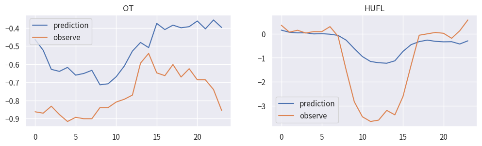
おおむね周期的な変化の傾向をとらえた予測ができています。しかし、論文Appendix Eに示されるきれいな予測結果を得るには、ハイパーパラメーターチューニングが必要そうです。

まとめ

Transfomerベースの時系列予測モデル、Informerを紹介しました。Informerは、ProbSparse self-attention, self-attention distilling, 生成的decoderを組み合わせることで、Transfomerの計算量の多さを軽減し、多変量長期時系列予測を可能にしたモデルです。

2023年時点では、Informerよりもよい精度で予測可能と主張する様々な後続論文が多数発表[3] [4]されていますが、いずれにおいてもInformerはベースラインモデルとして重要な役割を果たしています。

本稿では、理解のために著者実装をベースにJupyterNotebook上にべた書きしましたが、最近ではライブラリ実装もされてきています。例えば、ニューラルネットワークベースの時系列予測モデルが多数実装されているneuralforecastがあります。タスクによっては重厚長大な場合もありますが、このようなライブラリ実装を試してみるのもいいかもしれません。

---

[1]

Zhou, Haoyi, et al. "Informer: Beyond efficient transformer for long sequence time-series forecasting." Proceedings of the AAAI Conference on Artificial Intelligence. Vol. 35. No. 12. 2021.

[2]

Vaswani, Ashish, et al. "Attention is all you need." Advances in neural information processing systems 30 (2017).

[3]

Challu, Cristian, et al. “N-hits: Neural hierarchical interpolation for time series forecasting”. Accepted at the Thirty-Seventh AAAI Conference on Artificial Intelligence (2023).

[4]

Yue, Zhihan, et al. "Ts2vec: Towards universal representation of time series." Proceedings of the AAAI Conference on Artificial Intelligence. Vol. 36. No. 8. 2022.